Find systemmatricens egenværdier og tilhørende egenrum, og opstil ved hjælp heraf den fuldstændige reelle løsning på differentialligningssystemet.
Find den løsning på differentialligningssystemet som opfylder $\,x_1(0)=0\,$ og $\,x_2(0)=3\,.$
answer
Egenrummene er E$_3=$span${(4,1)}\,$ og E$_{-3}=$span${(-2,1)}\,.$ Alle multipliciteter er 1.
Den fuldstændige reelle løsning kan dermed opskrives som:
Find systemmatricens egenværdier og tilhørende egenrum, og opstil ved hjælp heraf den fuldstændige komplekse løsning på differentialligningssystemet.
Opstil nu den fuldstændige reelle løsning på differentialligningssystemet.
Vi skal nu finde den løsning på differentialligningssystemet som opfylder $\,x_1(0)=0\,$ og $\,x_2(0)=3\,.$ Overvej følgende: Får vi det samme resultat hvis vi finder løsningen ved hjælp af den fuldstændige komplekse løsning som ved hjælp af den fuldstændige reelle løsning?
answer
Egenrummene er E$_i=$span${(2+i,1)}\,$ og E$_{-i}=$span${(2-i,1)}\,.$ Alle multipliciteter er 1.
Den fuldstændige reelle løsning:
$$ \begin{matr}{rr} x_1(t) \newline x_2(t) \end{matr} = c_1 \begin{matr}{rr} 2\cos t-\sin t \newline \cos t \end{matr} + c_2 \begin{matr}{rr} \cos t + 2\sin t \newline \sin t \end{matr} , \quad (c_1,c_2) \in \reel^2$$
Find systemmatricens egenværdier og tilhørende egenrum, og opstil ved hjælp heraf den fuldstændige reelle løsning på differentialligningssystemet.
Find den løsning på differentialligningssystemet som opfylder $\,x_1(0)=0\,$ og $\,x_2(0)=3\,.$
answer
Kun ét egenrum som er E$_0=$span${(-\frac{1}{2},1)}\,.$ Multipliciteterne: am(0)=2. gm(0)=1. Kan ikke diagonaliseres ved similartransformation.
Den fuldstændige reelle løsning:
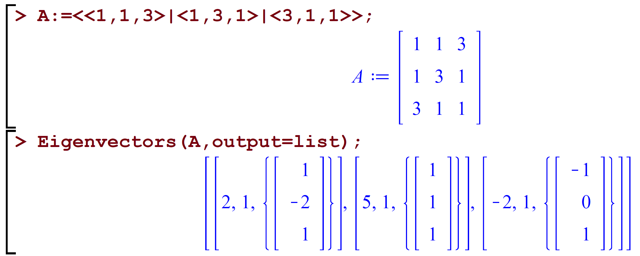
Et homogent lineært differentialligningssystem bestående af tre ligninger med tre ukendte funktioner $\,x_1(t),x_2(t)\,$ og $\,x_3(t)\,$ (med $t\in\reel$) har systemmatricen $\mA$ som har været behandlet i Maple/SymPy således:
\
\\Maple:
Hvordan ser de tre differentialligninger ud på sædvanlig vis (ikke matrixform).
B
Opskriv den fuldstændige reelle løsning på både vektorform og på sædvanlig vis.
Opg 3: Struktursætning. Teori
Lad $\,C^{\infty}(\Bbb R,\Bbb C))\,$ betegne funktionsvektorrummet af uendeligt mange gange differentiable komplekse funktioner af reel variabel med $\,\Bbb C\,$ som tilhørende skalar-legeme. For $\,t\in \reel\,$ er funktionerne $\,\cos(t),\,\e^{2it}\,$ og $\,t^3\,$ eksempler på vektorer i vektorrummet. Vi betragter nu afbildningen $\,f:(C^{\infty}(\Bbb R, \Bbb C))^2\rightarrow (C^{\infty}(\Bbb R,\Bbb C))^2\,$ givet ved
og opstil derefter den fuldstændige reelle løsning til differentialligningssystemet.
hint
Vedrørende gættet: Find først $\,x_2(t)\,$ ved at gætte på et førstegradspolynomium $\,at+b\,$ i nederste ligning. Indsæt resultatet i øverste ligning, og find nu $\,x_1(t)\,$ ved igen at gætte på et førstegradspolynomium.
Opskriv differentialligningssystemet på matrixform (som i spørgsmål b i forrige opgave). Find egenvektorerne og tilhørende egenværdi for systemmatricen.
B
Find med Maple/SymPy’s dsolve den fuldstændige løsning til differentialligningssystemet. Hvordan kan løsningen fortolkes, dels i lyset af egenvektorværdier og egenvektorer for systemmatricen, dels i lyset af struktursætningen?
C
Plot den løsning som opfylder $\,x_1(0)=10\,$ og $\,x_2(0)=5\,,$ først for $\,t\in \left[\,0,10\,\right]\,$ dernæst for $\,t\in \left[\,10,20\,\right]\,$ og kommentér resultatet.
Opg 6: Eksistens og entydighed. Teori.
Vi ser igen på det følgende differentialligningssystem fra opgave 1:
Gør rede for, at der til ethvert talsæt $(t_0,a_0,b_0)$ eksisterer netop én løsning $(x_1(t),x_2(t))$ til differentialligningssystemet således, at $x_1(t_0)=a_0$ og $x_2(t_0)=b_0$.
hint
Er det muligt at finde to forskellige løsninger, der opfylder $\,x_1(t_0)=a_0\,$ og $\,x_2(t_0)=b_0\,$?
hint
Indsæt $\,x_1(t_0)=a_0\,$ og $\,x_2(t_0)=b_0\,$ i den fundne fuldstændige løsning til differentialligningssystemet. Hvor mange forskellige værdier kan $\,c_1\,$ og $\,c_2\,$ antage?
hint
$\,c_1\,$ og $\,c_2\,$ er entydige. Hvorfor?
hint
Betragt den fundne fuldstændige løsning som et ligningssystem, hvor $\,c_1\,$ og $\,c_2\,$ er ubekendte. Vis, at der kun findes een løsning (koefficientmatricen er regulær).
$c_1$ og $c_2$ er entydigt bestemt og afhænger af talsættet $(t_0, a_0, b_0)$.
B
Givet et vilkårligt talsæt $\,(t_0,a_0,b_0)\,$. Overvej om der altid for differentialligningssystemer af de typer der er betragtet i opgaven ovenfor, eksisterer netop én løsning $\,(x_1(t),x_2(t))\,$ til differentialligningssystemet således, at $x_1(t_0)=a_0$ og $x_2(t_0)=b_0$.